Conditional formatting is a handy tool that changes the appearance of a cell or its contents based on specific conditions. This is a great way to make certain data in your spreadsheet stand out.
In Numbers, the Conditional Highlighting feature is what you’ll use to emphasize your data in this way. It’s super easy to use and once you get the hang of it, you’ll likely find yourself using it more and more.
This tutorial walks you through how to set up conditional formatting in Numbers for iPad for numbers, text, dates, and other data. Plus, we have some terrific tips to take your Conditional Highlighting to the next level.
When using spreadsheets, you’re likely to have more numbers than any other type of data. So, we’ll start by setting up Conditional Highlighting for numbers.
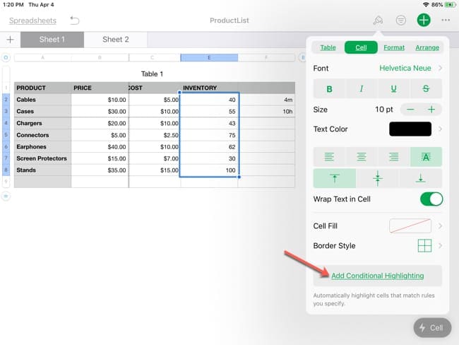
Let’s say you have a product list spreadsheet containing inventory. Whenever inventory gets low, you want to be alerted when you view the sheet.
Select the cells, row, or column containing the number you want to highlight.
Tap the Format button on the top right and select Cell.
Tap Add Conditional Highlighting at the bottom.
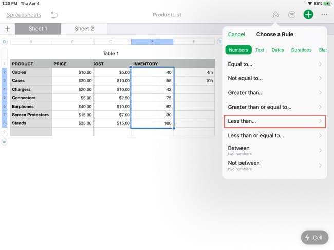
Under Choose a Rule, pick Numbers.
Add a conditional highlighting rule.
As you can see, you have a variety of options for creating your rule for numbers like Is equal to, Greater than, Less than, or Between. Select the one that applies; we’ll pick Less than.
Select the numbers rule type.
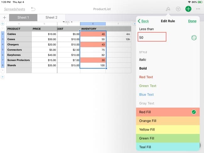
On the Edit Rule screen, enter the condition. For our example, we want to see when inventory is less than 50 units. So, we’ll enter 50.
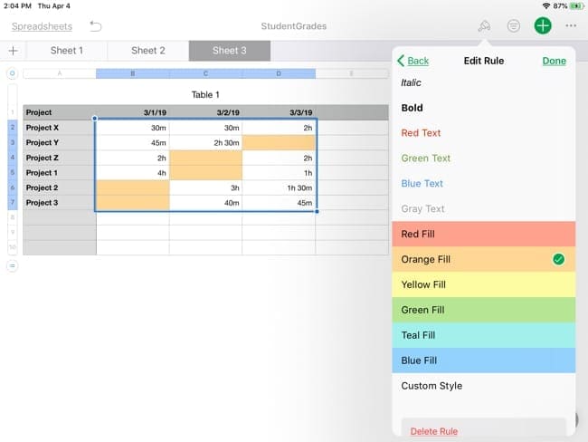
Then, scroll down and select the action for the condition. You can have the text stand out with italics, bold, or a certain color or have the cells highlighted with a specific color. If you prefer to create your own appearance, you can pick Custom Style to set it up.
We’re going to choose Red Fill for our spreadsheet. Tap Done when you finish setting up your rule.
Enter the condition and pick a highlighting type for numbers.
Now you will see that conditional formatting appear for the cells you chose.
Set up conditional formatting for text
Maybe for the data you’re using, you want certain text to stand out. And perhaps you want more than one Conditional Highlighting rule.
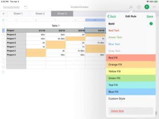
For this example, we have a grade sheet for school. When a student receives an A we want it highlighted in yellow and for an F we want it highlighted in orange so that both pop out at us.
Select the cells, row, or column containing the text you want to highlight.
Tap the Format button on the top right and select Cell.
Tap Add Conditional Highlighting at the bottom.
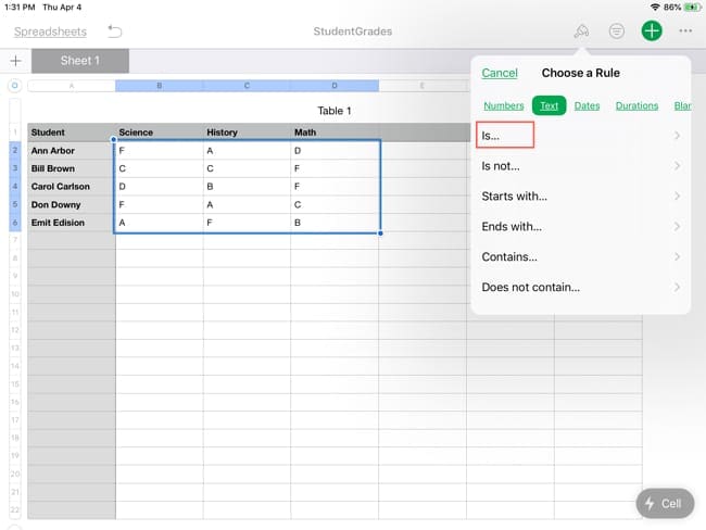
Under Choose a Rule, pick Text.
Select the text rule type.
Here again, you have many options for the conditions you want to use such as Is, Is not, Starts with, and Ends with. We’re going to pick Is because we want an exact match.
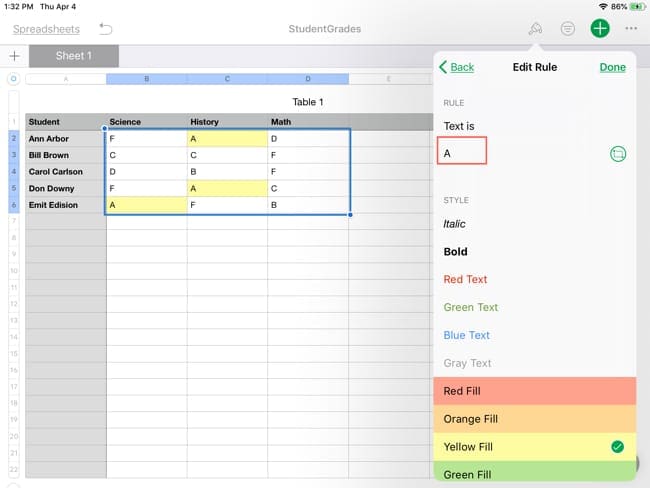
On the Edit Rule screen, enter the condition. For our example, we want to see when A student receives an A. So, we’ll enter A. Then, we’ll scroll down and choose Yellow Fill for our spreadsheet and tap Done.
Enter the condition and pick a highlighting type for the first text rule.
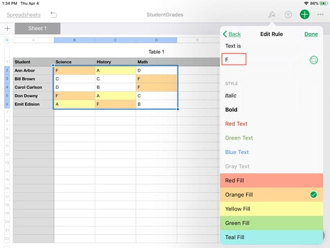
The format window should still be open at this time, so we’ll enter our second rule. Tap Add Rule at the bottom under the first rule. Go through the same process by selecting Is, entering an F this time, and picking Orange Fill. Tap Done.
Enter the condition and pick a highlighting type for the second text rule
You’ll see that both rules apply now and we can see those A’s and F’s clearly.
Set up conditional formatting for dates
If you use dates in your spreadsheets, it’s ideal to use Conditional Highlighting for showing upcoming dates, those that are past the due date, or items that fall within a certain date range.
Let’s say you keep track of your bills with Numbers and want to look at everything that was paid during a certain date range.
Select the cells, row, or column containing the dates you want to highlight.
Tap the Format button on the top right and select Cell.
Tap Add Conditional Highlighting at the bottom.
Under Choose a Rule, pick Dates.
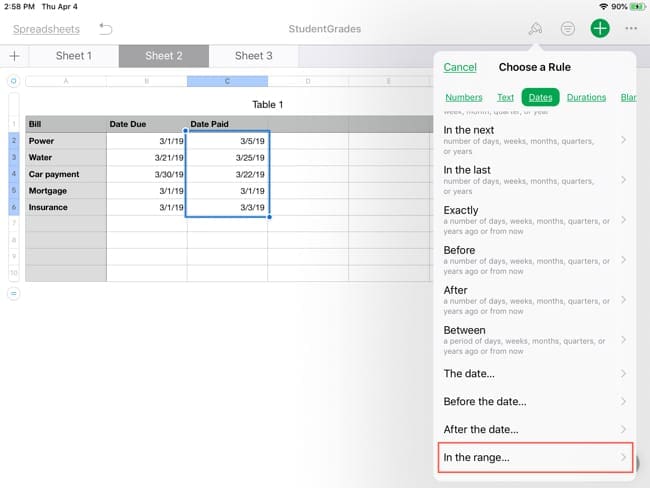
Select the dates rule type.
Conditional Highlighting for dates comes with many options from Today, Yesterday, and Tomorrow to Before, After, and In the range. These options give you a ton of flexibility.
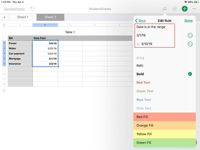
For our example, we’ll pick In the range. Next, we’ll enter the date range we want to use and pick the text or highlighting we want to apply. In our case, the range is March 1 through March 10 and the appearance will be bold text. Tap Done and then see the formatting immediately.
Enter the condition and pick a highlighting type for dates.
Set up conditional formatting for durations
Along with tracking dates in Numbers, you can track times and durations as well. You might use a spreadsheet to log workouts, tasks, or another activity that uses a period of time. Here’s how to apply Conditional Highlighting to durations.
Let’s say you keep track of projects and want to see which projects you spent two or more hours on each day.
Select the cells, row, or column containing the durations you want to highlight.
Tap the Format button on the top right and select Cell.
Tap Add Conditional Highlighting at the bottom.
Under Choose a Rule, pick Durations.
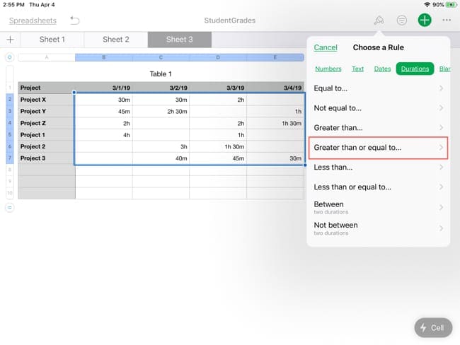
Select the durations rule type.
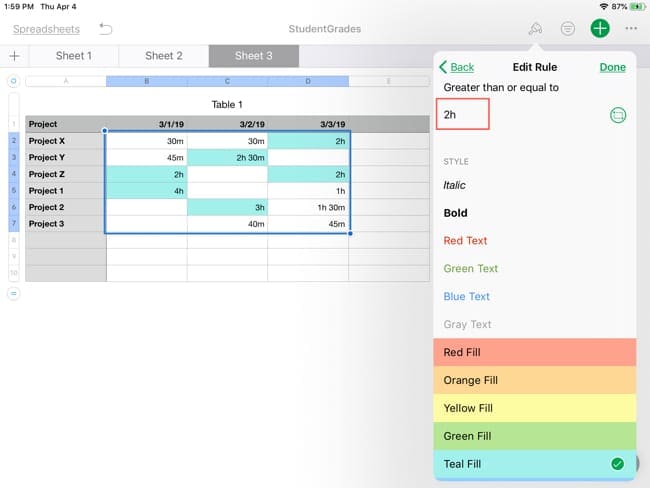
Durations gives you similar options as numbers like Equal to, Greater than, Less than, and Between. We’re going to choose Greater than or equal to and then enter two hours (which will display as 2h). Finally, we’ll pick Teal Fill and tap Done.
Enter the condition and pick a highlighting type for durations.
Any project that we spent two or more hours doing will be highlighted and easy to spot.
Set up conditional formatting for blank cells
Another good conditional formatting for spreadsheets, especially those you collaborate on, is for blank cells. This can alert you to missing data at a glance.
For the sake of our tutorial, we’ll use our projects spreadsheet again and color all blank cells orange.
Select the cells, row, or column containing the blank you want to highlight.
Tap the Format button on the top right and select Cell.
Tap Add Conditional Highlighting at the bottom.
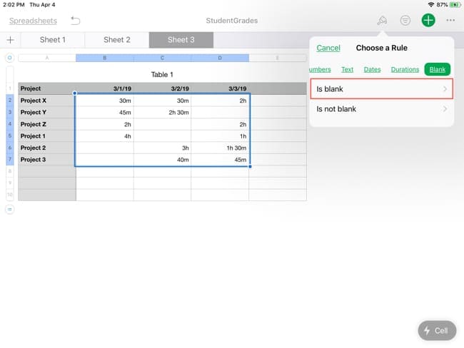
Under Choose a Rule, pick Blank.
Select the blanks rule type.
For this one, you only have two options Is blank and Is not blank. Obviously, we’ll pick Is blank for our project sheet. So, you won’t be entering any other conditions because a cell can only be full or empty. Just pick the highlight, ours is Orange fill, and tap Done.
Enter the condition and pick a highlighting type for blanks.
Now you can easily see any blank cells on your spreadsheet and make sure to get that data entered.
Do more with Conditional Highlighting
As you can see, conditional formatting in Numbers for iPad is flexible and simple. But there is even more you can do with it.
Repeat a highlighting rule
Maybe when you set up your spreadsheet, you didn’t anticipate adding more data or more data that might apply to the rules you set up. You can easily repeat a highlighting rule without manually setting it up for the new data.
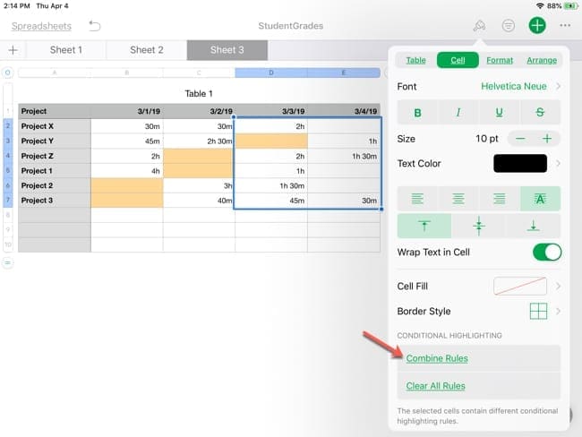
Select the cell containing the rule you set up along with the cell(s) you want the rule to also apply to.
Tap the Format button on the top right and select Cell.
Tap Combine Rules at the bottom.
Combine rules to make them repeat.
Now that same conditional formatting you set up before will apply to the additional data you added.
Use cell references and repeating rules
When adding the conditions to a rule, you can use a cell reference instead of typing in a number, text, date, or duration. The cell reference button is right below where you would enter your condition.
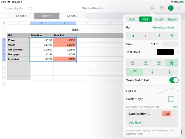
Using our bills example, let’s say we track the due date and date paid. Now we want to call out all of the bills that were paid late – after the due date. So, we’ll set up the rule and make it repeat to the other cells.
Select the first cell containing the date paid.
Tap the Format button on the top right and select Cell.
Tap Add Conditional Highlighting at the bottom.
Under Choose a Rule, pick Dates.
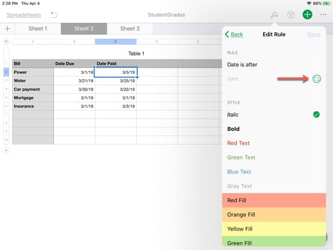
Use a cell reference for your rule condition
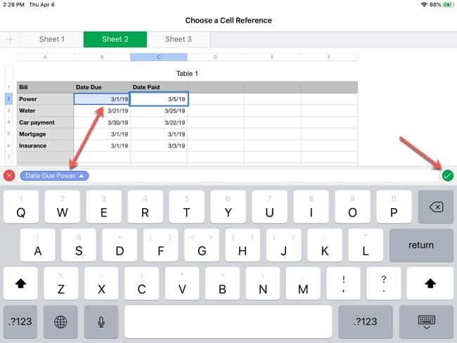
For the condition, we’ll pick After the date. Instead of typing in a date, tap the cell reference button. Then tap the cell containing the date due. Tap the checkmark in green, select your highlighting, and tap Done.
Enter the cell reference for the rule and click the checkmark.
Next, we want to apply that formatting to all bills that were past due.
Select the cell containing the rule you just set up and the cells below it where you want it to apply.
Tap the Format button on the top right and select Cell.
Tap Combine Rules at the bottom.
Combine rules and use a cell reference together.
Now you’ll see that all bills paid after the due date are highlighted in red.
Delete Conditional Highlighting
If you want to remove rules you set up for Conditional Highlighting, you have a few ways to do it.
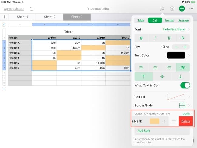
Select the cell(s) with the rule, tap the Format button, tap Edit, tap the minus sign, and finally, tap Delete.
Select the cell(s) with the rule, tap the rule, scroll to the bottom of the Edit Rule screen, and tap Delete Rule.
If it’s a combined rule, select the cells, tap the Format button, and tap Clear All Rules.
Delete a conditional highlighting rule.
Make data pop with conditional formatting in Numbers for iPad
Conditional formatting in Numbers for iPad gives you an easy way to make your data pop. Whether it’s numbers, text, dates, durations, or blanks, this convenient tool can help you zip through your spreadsheets for the data you want quickly and at a glance.
Are you going to set up conditional formatting for Numbers on iPad? If so, let us know which type you’ll be using. Feel free to leave a comment below or visit us on Twitter.
Sandy worked for many years in the IT industry as a project manager, department manager, and PMO Lead. She then decided to follow her dream and now writes about technology full-time. Sandy holds a Bachelors of Science in Information Technology.
She loves technology– specifically – terrific games and apps for iOS, software that makes your life easier, and productivity tools that you can use every day, in both work and home environments.
Her articles have regularly been featured at MakeUseOf, iDownloadBlog and many other leading tech publications.
Hi! Thank you for this post! Could someone please tell me if there’s a way to add a conditional formatting based on another cell’s value? E.g., if cell A1= 1, then cell B1’s text should be in italic.
Sandy,
Thanks.
I keep over-thinking how Numbers works. e.g. I knew that in other spreadsheets, TRUE and FALSE are actually 1 and 0, so I thought I needed to use a Number-based conditional format, which didn’t work. I swapped to using a Text-based format, and that worked perfectly.


Hi!
I’m just learning NUMBERS on iPad, and I can’t figure out how to highlight ODD or EVEN numbers.
Thanks
Hi! Thank you for this post! Could someone please tell me if there’s a way to add a conditional formatting based on another cell’s value? E.g., if cell A1= 1, then cell B1’s text should be in italic.
This information is very helpful and easy to follow.
Thank you
Sandy,
Thanks.
I keep over-thinking how Numbers works. e.g. I knew that in other spreadsheets, TRUE and FALSE are actually 1 and 0, so I thought I needed to use a Number-based conditional format, which didn’t work. I swapped to using a Text-based format, and that worked perfectly.
Can i know what app is this, is it a google product or from apple ? Thank you.
Hi Muhammad,
Numbers is an Apple App–available in the App Store at no cost.