A few weeks ago, we covered the basic techniques for using Numbers on Mac. In case you missed that post, we explored Numbers features like formulas, templates, sheets, and sorting.
Today, we’re going to expand on that post by covering more advanced techniques. If you aren’t familiar with the topics covered in that first post, I strongly suggest you read it before working through this one. For those that are getting comfortable with Numbers, however, and want to expand their working knowledge, then this post is for you.
In this post, we’re going to be looking at advanced techniques such as creating charts, pivot tables, adding filtering and conditional formatting, and exploring the possibilities of combining Numbers with AppleScript. This is going to be a bit of a “level up”, so get ready, and let’s get started!
The first thing we’re going to cover is a feature that’s relatively new to Numbers on Mac: Pivot tables. It used to be that this was a feature that only Excel users could enjoy. But in recent updates, Apple has brought pivot tables to Mac.
So what are pivot tables? For those that don’t know, a pivot table is sort of like a standard table of data, except that it is interactive. The interactive aspects of a pivot table allow you to quickly organize, filter through, sort, and better understand the data in your table.
For instance, in a typical Numbers table, you’ll see several rows and columns of data that, no matter how organized, is likely difficult to quickly take insights from. So you can map this table of data to a pivot table, which will quickly show you summaries of the data, show relationships between your data, and more.
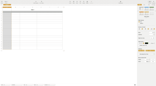
To create a pivot table in Numbers, you’ll first need a table or range of data. A range of data is just a row or column of data, while a table is a series of rows and columns.
Select your range or table, then click Pivot Table in the toolbar at the top of your screen. You’ll be asked to choose from one of these four options:
On New Sheet: This creates a new sheet containing your pivot table. This separates your table and pivot table visually to keep things organized.
On Current Sheet: This adds the pivot table to the sheet you’re currently using, allowing you to view your table and pivot table at the same time.
For Selected Cells on New Sheet: If you don’t want to create a pivot table using a table, you can instead select a range. If you choose this option, you’ll create a pivot table for your range on a new sheet.
For Selected Cells on Current Sheet: Lastly, as expected, this option takes your selected range of cells and creates a pivot table for them on your current Numbers sheet.
The best way to get the hang of pivot tables is to start creating and experimenting with them. We don’t have time in this post to go much more in-depth than this, but we will be doing a future post on pivot tables exploring them in more detail. So stay tuned for that!
Creating charts
The next advanced technique you’ll want to learn when using Numbers on Mac is creating charts. While charts aren’t strictly necessary when using Numbers, they’re a great visualization tool.
For those that aren’t familiar with charts, they’re a way of taking data in a table and displaying it in a more visual way. This is great for taking away quick insights as well as showing your data to non-technical individuals. For instance, if you have been keeping track of expenses in Numbers and need to show these expenses during a conference, you can create a chart and show it off in a presentation.
Creating a chart in Numbers is super easy. Just choose the Chart option from the toolbar and choose a 2D, 3D, or interactive chart for your dataset. If you aren’t sure what to go with, then it’s probably best to stick with a 2D option.
Again, we don’t have enough time in this post to go in-depth on chart creation. But in general, pie charts and bar charts are a great choice. Pie charts help show percentages and quantities, while bar charts are better for comparing things in a visual hierarchy.
Just as with pivot tables, it helps to experiment with the various chart options. So create a dataset and start making charts based on that dataset.
Also! One last piece of advice. When creating a chart that has an X and Y axis (bar charts, for instance, have this), try to keep constant numbers on the X axis and variable numbers on the Y axis. For example, it’s common practice to put time variables on the X axis (months, years, weeks, quarters, etc.) and financial values on the Y axis (currencies, earnings, expenses, losses, growth, etc.).
Conditional highlighting in Numbers on Mac
Another important technique to master in Numbers on Mac is conditional highlighting. As you may have noticed by now, you can format the content in your cells. You can change the background color of a cell, change the font color and type, and so on.
Like charts, formatting can be used to help visually organize your data. By color coding data entries, you can quickly distinguish between positive and negative values, dates and dollar amounts, clients, and so on.
Of course, changing all of this formatting manually can take up a lot of time. That’s where conditional highlighting comes in. It allows you to create automatic rules that instantly change the formatting of your cells. So if you have Clients A, B, and C, you could create rules so that all A entries are green, all B entries are blue, and all C entries are red.
To set up conditional highlighting rules, select a cell, range of cells, or an entire column/row. Then, click Format in the top-right of the Numbers screen. This should show (not hide) the Format panel on the right side of your screen.
At the top of this panel, select Cell. Then, click Conditional Highlighting…
Select Add a Rule. You can then create a rule that is based on numbers, text, dates, and so on. Each type of rule has its own parameters, so choose the one that best meets your needs. For instance, if you want every cell with the text “Client A” to be green, you would choose Text > Is…
You can, of course, change these rules to match your needs. If you set it up as I have, though, then any time you type “Client A” in a cell with these conditional highlighting rules, the background color will instantly become green.
To be clear, this doesn’t necessarily change the function of your data or your table. It just helps make things clear visually and saves you time.
Formatting numbers
Similar to conditional highlighting is formatting numbers in Numbers on Mac. By default, all of the numbers you enter into Numbers are going to look relatively similar. However, not all numbers should be formatted in the same way. You’ll have dates, times, currencies, and percentages.
To ensure that these numbers look the way that they’re meant to, you can set rules for the formatting of various cells and ranges. To set this up, you’re going to want to make sure that the Format sidebar is open, and you’re going to want to choose Cell in this sidebar again.
You’ll notice that near the top of this section of the sidebar is a dropdown menu labeled Data Format. When you select that dropdown menu, you’ll see the following options:
All you need to do from here is choose the formatting that you want to use for your selected cells. From then on out, your cells will automatically be formatted appropriately.
And if you choose Number from the dropdown menu, you can even choose the number of decimal places that are shown. This can be really helpful for displaying information the way you want it displayed.
Filtering
Another useful display option in Numbers on Mac is filtering. Filtering, similar to pivot tables, allows you to show only the information that is relevant to you. For example, you can use filtering to hide expenses you can’t afford, show only the clients you owe, or display all upcoming entries.
In other words, it allows you to fill in all of your data, then filter through it based on rules you choose.
When creating filtering rules, you have two options:
Quick Filters: These are automatically generated filtering rules that appear based on the data you’ve entered in your table. They’re useful when you just want to quickly filter out certain information and aren’t looking to necessarily organize your dataset in a particular way.
Filtering Rules: Filtering rules, on the other hand, are rules that you establish for your table/dataset. They’re more permanent, structured, and can be accessed whenever you need them.
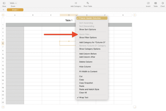
To use Quick Filters, select a column of data or a specific cell, hover over the corresponding column letter, then click the arrow that appears next to the column letter. This will bring up a dropdown menu, on which you will find Quick Filter options.
Select it, then choose from the available filtering options it presents to change the visible data. The data isn’t being deleted or changed, just hidden from view.
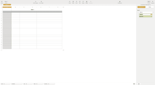
For filtering rules, select the column, row, or cells you want to filter. Then, right-click them and choose Show Filter Options.
Next, in the sidebar (which should have changed to show filtering options), you can add a filter to a column of your choosing. Just like with conditional highlighting, you can create rules that will allow you to show/hide data strategically.
Mastering COUNTIF in Numbers on Mac
One of the most powerful functions in Numbers on Mac is COUNTIF. Technically, there are other “IF” functions, but once you understand how COUNTIF works, you’ll be able to figure the rest out, too.
In essence, COUNTIF allows users to apply a formula to a range of numbers, but also to exclude numbers that don’t meet certain conditions. So you “COUNT” numbers “IF” they meet your conditions.
For example, you could use this to only count your sales that are greater than $100, ignore clients that have spent less than $10, or only look at payments that haven’t been processed.
To use a COUNTIF function, click Insert at the top of the screen, then Formula, then New Formula. This will change the sidebar to show all of the formulas available to you. In the search bar of this side panel, type “IF” and hit return.
When you do this, you’ll see functions like IF, SUMIF, AVERAGEIF, and of course, COUNTIF. These are all functions that take advantage of the IF feature, so just choose the one that applies to your needs.
You’ll notice that there are also “-IFS” functions. These work more or less the same way, except that they allow you to check multiple collections for multiple collections, rather than a single collection for a single condition.
Using VLOOKUP
Next is VLOOKUP. VLOOKUP is a staple feature of Excel, and it’s one that those using Numbers on Mac are going to want to get familiar with. Once you are, you’ll find yourself using this feature all of the time.
For those that don’t know, VLOOKUP is a function that allows you to look up a specific piece of data that corresponds to another piece of data. For example, you could look up the hourly rate (Column B) charged to a client (Column A).
From there, you can use the value that you’ve looked up in another function. So it’s a great way to start organizing and transposing pieces of data around your dataset.
To use VLOOKUP, you’re going to revisit the steps taken in the last technique we covered. Select Insert at the top of the screen, then choose Formula and New Formula. This should change your side panel to show the formula selection panel.
In this panel’s search bar, type “VLOOKUP” and press return on your keyboard. You should see VLOOKUP appear instantly.
Go ahead and select VLOOKUP to start creating the formula in a cell of your choosing.
To make this function work, you’re going to need to fill in the following pieces of information:
Search for: This is where you’ll enter the value that you want to find. You can enter a number or a REGEX string. If you aren’t familiar with REGEX, this post will get you up to speed.
Columns range: The next section is the selection of cells that you’re going to be searching through. So specify which cells you want to find the Search for content in.
Return column: The return column is where you’re going to specify what piece of data you want returned. For instance, if you’re looking for someone’s Hourly Pay (Column A), then you may want to actually pull the value contained in Column B, which has the dollar amount they earn. In other words, this is the value that will specify which piece of data this function will return.
Close match: This parameter allows you to choose how much leeway you give to the data your VLOOKUP formula finds. For instance, say you’re looking for the number “5.5” but the formula finds “5.6” instead. You can use Close match to decide if this would show up as an error or if you want to count it as being accurate enough.
And that’s it! VLOOKUP can be a bit tricky to get the hang of, but once you do it’ll be a truly powerful tool in your arsenal. So spend lots of time with it until you’re comfortable using it. I’ve found that Reddit communities for Excel and Numbers have a lot of insight into how VLOOKUP works, if you need some extra reading.
Collaborate with coworkers
One of the simplest advanced techniques we’re going to cover in this tutorial on Numbers on Mac is collaboration. In recent updates, Apple has added the ability for users to collaborate with one another in Numbers.
Doing this is a super easy and great way to make you and your team more productive. To do this, just click the Collaborate button in the toolbar and share access to your spreadsheet with others via email, text, or AirDrop.
The people you’re collaborating with will need to have an Apple device, preferably a Mac or iPad, though an iPhone will also work.
When collaborating on a Numbers file, you’ll be able to see the exact edits and contributions that others have made. This is great for sharing documents with people, working on the same file using different devices or at different times, and keeping your workplace team connected.
Adding AppleScript to Numbers
Last but not least, a pretty advanced technique for Numbers on Mac is using AppleScript with your spreadsheets. For those that don’t know, AppleScript is a basic scripting language from Apple that can be used to automate certain tasks.
For those that are familiar with Excel, you may have experience with macros. Macros allow you to automate basic tasks, like entering in numbers or updating information. It’s a great timesaver and one that is built into Excel.
Unfortunately, Apple hasn’t built in a similar feature to Numbers yet. Instead, you’ll need to rely on AppleScript.
The good news is that AppleScript is pretty simple. If you already have some programming experience then you should be able to pick it up pretty quickly. And if you don’t, you can either learn the basics or copy code that others have written online.
Like a lot of what’s in this article, we don’t have time to go on a deep dive of all of the things you can do with AppleScript in Numbers. Just know that if you find yourself doing a lot of repetitive tasks in Numbers, you can use AppleScript to start offloading that work onto your computer.
Numbers on Mac: Becoming a pro
And that’s it! By mastering the techniques outlined in this post, you can start sharpening your skills in Numbers on Mac and make progress towards becoming a true pro. While some of these concepts may be hard to wrap your head around at first, odds are good that you’ll wind up using a lot of this stuff on a daily basis.
These are great techniques to learn if you’re looking to work in Numbers or Excel for a living. And for those that just need Numbers for projects at home, this will enable you to do a whole host of new things. Let me know in the comments below how you plan to use these various techniques!


Write a Comment